Measurement and Uncertainties

Tutorial

Measurement and Uncertainties

Introduction

Uncertainties are present on all types of sensors. To quantify the uncertainties of the sensors, it is essential to consider the different factors of each uncertainty. First of all, it is important to distinguish an uncertainty from an error. An error, also misnamed accuracy, is the difference between the exact value and the measured value, but in all cases, the exact value is not known. The uncertainty, however, represents the spread of values that can reasonably be attributed to the measurement.

When accuracy is required, we have to ‘compare apples to apples’. This means that we have to understand what we are talking about regarding uncertainty and to define the confidence interval. A confidence interval is the range of values where our true value is expected to lie. From a statistical point of view: “The larger the confidence range the greater the uncertainty” is what we consider for a “normal” law.

There are 3 confidence interval sizes:

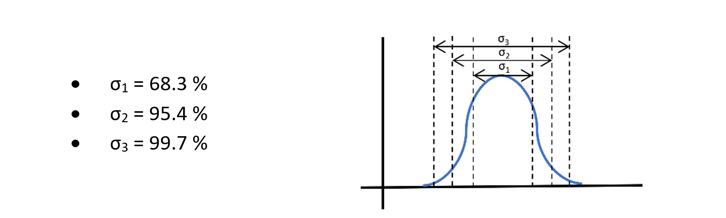
The quantity ‘σ’ represents the standard deviation of the measurement. It is important to understand that a lot of datasheets give accuracy values by mentioning the average value with a variation range equal to ‘σ_1′_.

In this tutorial we will summarize the different uncertainties that are encountered when calibrating a pressure sensor.

The following diagram shows the different elements that are necessary for a calibration. All calibrations require a reference pressure sensor that allows us to calibrate our sensors against it. A temperature sensor is particularly useful when we make calibrations at a specific temperature. Then, the power supply and the output signal of the elements are managed by an interface card whose components can have an impact on the measurement of the sensors. Furthermore, it is necessary to add to this calibration an acquisition equipment that allows to receive the data from all the sensors, as well as a power source that supplies them.

Each of these elements have uncertainties that have an impact on the tested pressure sensor, it’s the misnamed error/accuracy.

Sensorade Test Bench

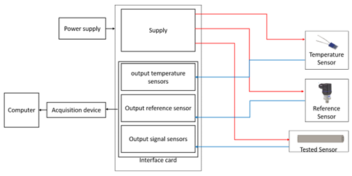
Figure 1: Sensorade Test Bench Set-up

2. The Uncertainties – elements of calibration

Please notice that this tutorial outlines uncertainties and does not show all the uncertainties taken into account during the calibrations on the Sensorade test bench.

In our case, it is necessary to determine the uncertainties of the above elements such as the pressure sensor, the acquisition system,… In order to determine these uncertainties, we must use the following equation (from the “Evaluation of measurement data —Guide to the expression of uncertainty in measurement”):

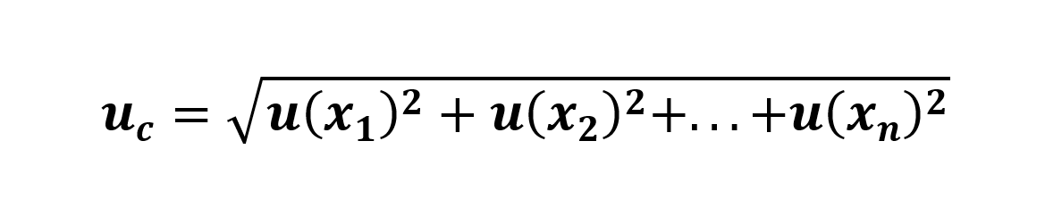
Equation 1: General Uncertainty

u_c represents the uncertainty we are looking for
u(x_i) represents the uncertainties that influence the uncertainty (e.g. the precision, the resolution,… of a sensor)

For a test bench, it is easy to understand that we must use the elements with the lowest possible uncertainties to reduce the uncertainty on the sensor itself. So we must know/calculate the uncertainties of the different elements of influence. Be advised that if this job is not done, you will not be able to expect any confidence on the tests performed.

Determination of Uncertainties

There are several methods to determine uncertainties. We particularly use two types of uncertainty determination : type A and type B.

Type A :

Type A uncertainty determines the uncertainty of an element by following a certain procedure. This procedure consists in measuring the signal of the element several times in a repeated and identical way. This often makes it possible to determine a much more precise uncertainty, but it is only applicable to one specific element.

Type B:

Type B consists in determining the uncertainty by using the documents / datasheet provided by the supplier. Unfortunately, not all manufacturers specify the uncertainties of their components, or some manufacturers provide the uncertainty on a batch of components, so the uncertainty can often be very large, too large. Therefore, if the uncertainty is not given by the manufacturer, it is mandatory to use the type A method. Moreover, the type A method must also be used if the uncertainty provided by the supplier is too large and covers a batch of the same component.

Let’s take an example: we want to determine the uncertainty of 5 resistors of 1000 Ω of the same reference with both methods.

Using Type A, we obtain the table below with the mean and standard deviation values:

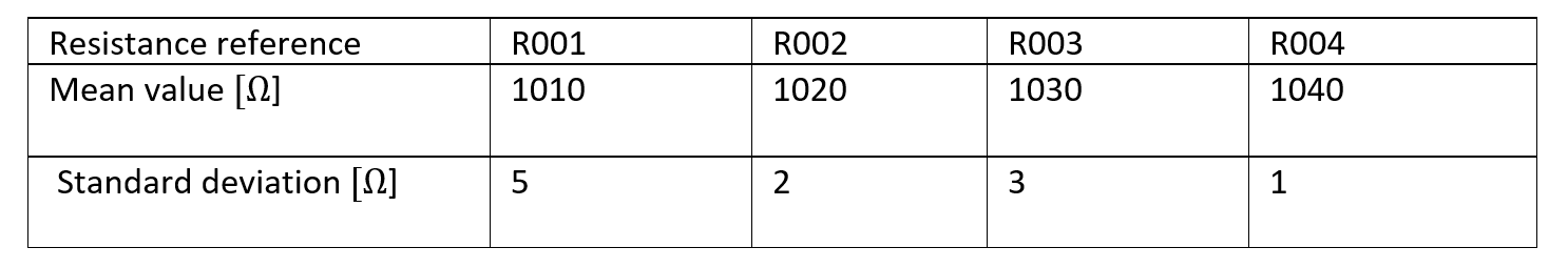
Using Type B we read the datasheet, and notice that the precision is 5%, so the uncertainty of the 5 resistors would be 5%.

On this example, we can notice that the resistor R004 has the lowest standard deviation but the highest mean value. So, if we modify – where it is allowed – the value of the resistor from 1000 by 1040 in the calculation, we can decrease the uncertainty by a factor of 5 (type B) by 0.1% (type A). But this uncertainty would only be valid for the resistor R004.

In our case, it is necessary to apply this determination of uncertainty to determine the uncertainty of the elements of influence which are the reference sensor, the temperature sensor, the acquisition card and various components on the interface card.

If several uncertainties occur for an element, it is necessary to apply Equation 1 (General uncertainty) before applying this equation. It is important to check that all the uncertainties are given in the same confidence interval and that they follow a standard law, otherwise the calculation would be wrong.

Once the uncertainties of the different elements of influence are determined, it is necessary to be able to combine them in order to determine the uncertainty of the pressure sensor under test. To quantify the impact of the influence elements on the sensor, it is necessary to know the best fitted linear equation of the pressure sensor.

3. The Pressure Sensor Model

Pressure sensors are governed by a linear equation that relates the applied pressure to the output and supply voltage.

We can therefore see by Equation 2 that two parameters, a and b, must be determined. To do this, we use a linear model which, with the help of calibration data, allows us to determine them. We will not detail these calculations in this tutorial.

Important remark: Theoretically speaking, a and b are constant, but in fact, a and b are temperature-dependent (at least). It means that you need to have the full control on your environment.

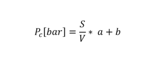
Equation 2: Pressure Sensor

S = (sensor output signal voltage)
V = (sensor supply voltage)
a = the slope of the line
b = y-intercept

A. Model Uncertainty

The fact of using a model, introduces a new uncertainty which is the uncertainty of the model. This uncertainty changes according to the selected model. This is more or less complex according to the complexity of the model.

The graph here on the right illustrates where this uncertainty comes from. On the ordinate, we see the applied pressure and on the abscissa, the S/V ratio which represents the ratio between the output voltage and the supply voltage. The curve in red represents the linear model of the sensor.

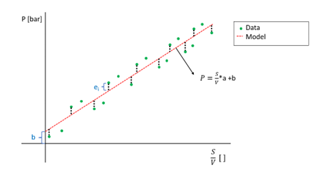
Figure 2: Model Uncertainty

For that reason, it is normal that the use of a model introduces uncertainties because when a model is used, the set of data points does not lie perfectly on the model. It is from there that the uncertainty of the model comes. The determination of this uncertainty is done by calculations given by the selected model, therefore we will not go into the details.

On the other hand, it is possible to have an idea of the uncertainty of the model by means of a simple calculation which makes it possible to quantify the validity of a model. It is the calculation of the coefficient of determination, determined by the equation below:

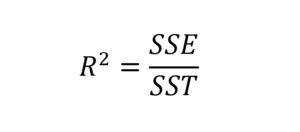
Equation 3: Model Quality

SSE = model variation
SST = total change
R = coefficient of determination, the closer it is to 1, the more the model represents the data

For our Sensorade sensors, the coefficient of determination is close to 0.999. This proves that the model we use is very close to reality.

B. Determination of the uncertainty of the pressure sensor

To determine the uncertainty of the pressure sensor, another equation must be used that combines the different uncertainties of elements of influence (from the “Evaluation of measurement data —Guide to the expression of uncertainty in measurement”):

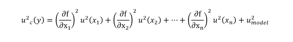
Equation 4: General Uncertainty for the Functions

u_c represents the uncertainty we are looking for
Xi is a variable of the equation (Ex: the parameter S, Equation 2)
u(Xi) represents the uncertainty of an element of influence
Umodel represents the uncertainty of the model
f is the linear function that represents the data (e.g. the equation P_c, Equation 2)
(∂f/∂X1)² represents the partial derivatives

The last step is to apply Equation 4 since all the terms have been determined in the previous sections. Finally, we obtain the uncertainty value of our pressure sensors.

4. Conclusion :

In conclusion, uncertainties are present in each component of the test bench, from all acquisition devices, elements, connectors… to the sensor you want to calibrate.

Therefore, to determine the uncertainty of our sensors, we must first determine the uncertainties of the elements of influence by applying the method of type A or B, according to the elements and the data provided.

Then, the linear model of the sensor and the uncertainty of the model must be evaluated. We can notice that the main uncertainties come from the elements that are external to the pressure sensor, in particular the acquisition system.

Finally, the uncertainties of the element of influence and of the model should be combined in order to determine the calibration uncertainty of our sensors.

Discover our products